Overview

Energy Measurement records and analyzes the current, voltage, power, and accumulated energy of a target MCU. Measurements are obtained through an NXP standalone MCU-Link Pro debug probe or another MCU-Link-based on-board probe.

It offers a command-line reporting mode for automated/CI use and an interactive graphical interface for live visualization and detailed analysis. The graphical interface can be opened as a standalone window with ./LinkServer measure gui, or served to a web browser with ./LinkServer measure server.

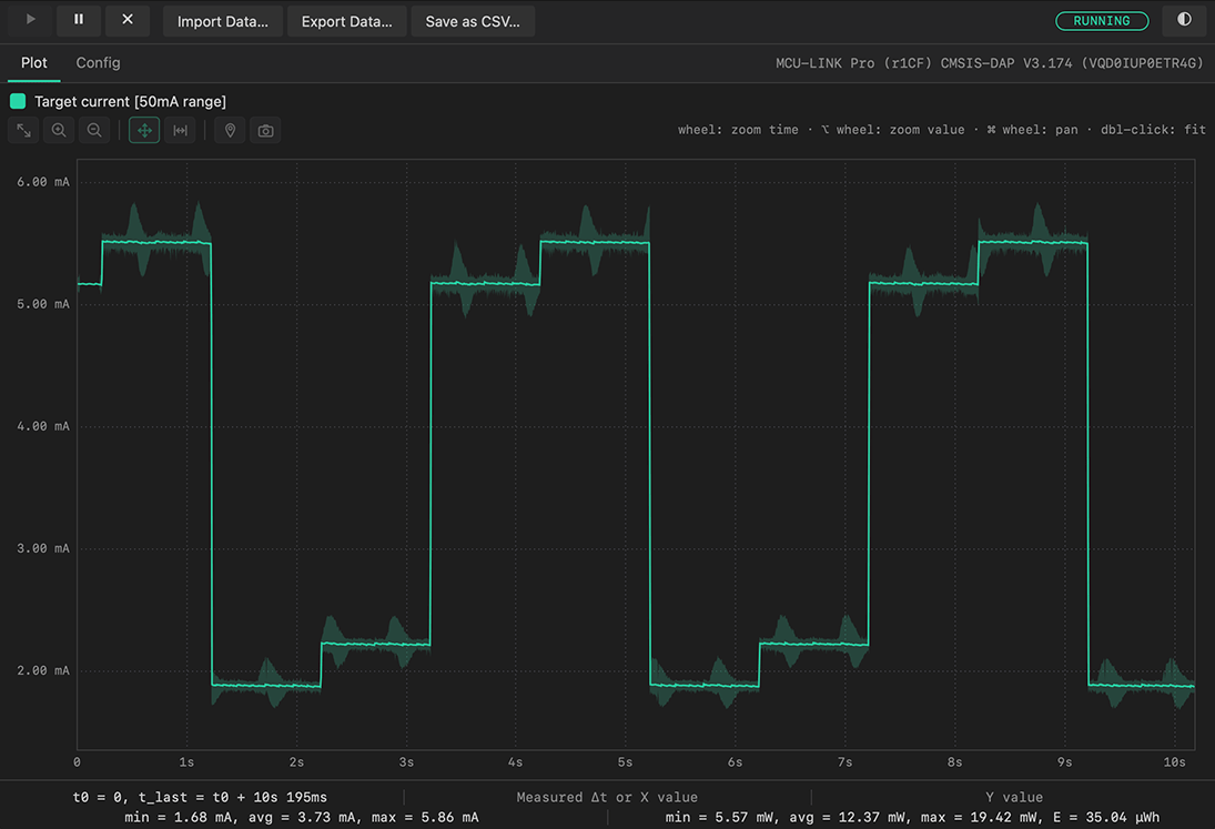
This document describes the functionality provided by Energy Measurement.

Requirements

• A power-capable probe, for example, the MCU-Link Pro connected to the target through its energy-measurement header.

• A target board (or on-board device) powered through the probe’s measurement path so that the probe can sense the target current.

If more than one probe is connected, select the one to use with the --probe option (see Common options).

To analyze a previously captured archive without a probe connected, use offline mode, available in all three subcommands.

On Linux, the standalone GUI window (measure gui) is rendered with the system WebKitGTK runtime. On Debian or Ubuntu, install the required packages with sudo apt install gir1.2-webkit2-4.1 libwebkit2gtk-4.1-0 if needed. If WebKitGTK is unavailable, measure gui automatically opens the interface in your default web browser. The measure server always uses a browser. On Windows and macOS, the built-in web view is used and therefore, no other installation is required.

Modes

Energy Measurement is invoked through the measure command, which provides three subcommands listed in the following Table.

Command	Description
./LinkServer measure report	Command-line capture that prints a summary (and optional periodic report) and can write the captured data to a file. Suitable for scripting and CI. Optionally, it replays a previously saved archive instead of capturing, see offline mode.
./LinkServer measure gui	Open the interactive graphical interface in a standalone window. Also available as ./LinkServer gui measure.
./LinkServer measure server	Start a local HTTP server that serves the same graphical interface to a web browser (useful for headless hosts, remote access, or integration into other tools).

Use ./LinkServer measure <subcommand> --help for the full list of options of each subcommand.

Common options

The following options are available for all three subcommands and determine the initial measurement configuration. In graphical modes, they pre-fill the Config tab and can be modified in the UI before the measurement begins. In report mode, they are applied directly to the capture.

Option	Description
-s, --source	Source to measure: current, voltage, power, dbg_vref (debug interface reference voltage), or analog_input.
-r, --rate	Sampling rate in samples/second: 10000, 25000, 50000 (default), 62500, or 100000.
-v, --voltage VOLTS|auto	Target voltage used to derive power and energy from a current measurement. Provide a fixed value in volts, or auto to read the target-voltage source briefly before the capture starts.
-t, --time SECONDS	Automatically stop the capture after the specified number of seconds. Fractional values are supported, such as 0.5. If omitted, the capture continues until you stop it manually by pressing Ctrl+C in report mode or selecting Pause or Clear in the UI.
-f, --filter SPEC	Apply a noise filter to the samples: maf:WINDOW (moving average), amf:WINDOW (arithmetic mean), folpa:ALPHA (first-order low-pass), or kalman:Q[:R]. Example: maf:16. Default: no filtering.
--trigger	Gate the measurement on a probe input signal: level-high / level-low (measure while the signal is high/low) or pulse-high / pulse-low (each pulse toggles measurement on/off).
--trigger-initial	Whether the measurement is active before the first trigger edge/pulse: disabled (default) or enabled.
-p, --probe TEXT	Probe to use, by serial-number substring or by index (for example --probe '#1'). Only needed when more than one probe is connected.

CLI reporting mode (report)

./LinkServer measure report performs a capture without a UI, prints a summary when it finishes, and can optionally emit a periodic status line and/or save the captured data.

More options:

Option	Description
-i, --report-interval SECONDS	Print a status line every N seconds while capturing.
--no-summary	Do not print the final summary report.
--output-csv FILE	Write the scaled sample values to a CSV file (a timestamp_us column and the value; a power_W column is added when a target voltage is available).
--output-bin FILE	Write the captured data as an Energy Measurement .zip archive (raw binary data plus a configuration descriptor) that can later be opened in the graphical interface with Import Data.
--offline ARCHIVE	Report on a previously saved Energy Measurement .zip archive instead of measuring; no probe involved. See Offline mode.

To write both files from a single capture, specify both --output-csv and --output-bin.

When the capture starts, a single line announces what is being measured:

Measuring Target current [50 mA range] (@ 50000 samples/s) until Ctrl-C with periodic report each 1s.

Periodic report

With --report-interval N, a status line is printed every N seconds of captured time (can be fractional like 0.2).

Each line is split into two parts by |:

• Per-interval (left): The average of the measured quantity over that interval only. For a current source with a target voltage, the average power of the interval (interval-average current × target voltage) is shown right beside it.

• Total: accumulated (right): The minimum/average/maximum of the measured quantity since the start of the capture. For a current source with a target voltage, it also appends the overall average power P (global-average current × target voltage) and the accumulated energy E.

The leading [  start..  end s] is the time window of the interval, relative to the start of the capture. The exact fields depend on the source:

Current with a target voltage (--source current --voltage 3.3) — per-interval current and power on the left; accumulated min/avg/max, overall average power, and energy on the right:

[   2.400..   2.700s]:   5.58 mA,  18.41 mW  |  Total: min =   1.86 mA, avg =   3.83 mA, max =   5.84 mA, P =  12.64 mW,  E =   9.49 µWh

Current without a target voltage — no power or energy is derived:

[   2.400..   2.700s]:   5.58 mA  |  Total: min =   1.86 mA, avg =   3.83 mA, max =   5.84 mA

Power source (--source power) — the value is power already, therefore, the accumulated energy E is added:

[   1.200..   1.500s]:  17.45 mW  |  Total: min =   7.14 mW, avg =  14.40 mW, max =  18.65 mW,  E =   6.01 µWh

Voltage source (--source voltage) — only min/avg/max:

[   2.400..   2.700s]:   3.30 V  |  Total: min =   3.29 V, avg =   3.30 V, max =   3.31 V

Final summary

Unless --no-summary is given, a summary is printed when the capture ends. The summary contains a single block showing the measured source with its duration and sample count, the min/avg/max values. For a current source with a target voltage, it also includes the corresponding power figures, with the voltage used shown in parentheses and the total accumulated energy E:

Target current [50 mA range] duration: 3.465 s (173228 samples)
  min = 1.86 mA,  avg = 4.05 mA,  max = 5.84 mA
  min = 6.16 mW,  avg = 13.37 mW,  max = 19.28 mW  (3.30 V)
  E = 12.88 µWh

Examples:

• Measure the target current for 5 seconds at 50 kHz (default) and print the summary:
  ./LinkServer measure report --source current --time 5

• Measure current with power/energy derived from a 3.3 V rail, printing a status line every half-second:
  ./LinkServer measure report --source current --voltage 3.3 --report-interval 0.5

• Capture until Ctrl-C and save an archive for later analysis in the GUI:
  ./LinkServer measure report --source current --voltage auto --output-bin session.zip

• Capture a fixed window and export scaled samples as CSV:
  ./LinkServer measure report --source current --voltage 3.3 --time 10 --output-csv session.csv

• Report on a previously captured archive, with no probe connected:
  ./LinkServer measure report --offline session.zip

Interactive graphical interface (gui / server)

The gui and server subcommands present the same interface. gui opens it in a native window; server prints a local URL to open in a browser:

INFO: Interactive measure server at http://127.0.0.1:PORT/ — connect a browser (Ctrl-C to stop)

The server listens on the loopback interface only, and its /api endpoints are protected by an access token generated at start. The page served at the URL above carries that token, so opening it in a browser needs no extra step. Two options help when another tool drives the server:

Option	Description
--port PORT	Listen on a fixed port instead of letting the system pick a free one, so the URL is predictable.
--json	Print a single JSON line with the server URL and the access token before starting, for tooling that embeds the interface. For example, a VS Code webview.

When launched, the interface connects to the probe but does not start measuring automatically. You configure the parameters and control the capture from the UI.

The window is organized as a top toolbar and two tabs: Config and Plot. During a live session, the connected probe’s name and serial number are shown at the right end of the tab bar. As a result, the active probe stays identifiable from either tab.

Toolbar

The toolbar is available from both tabs.

• ▶ Play: Start a new measurement (or resume a paused one) using the current configuration. Changing configuration and pressing Play again restarts the measurement with the new settings.

• ⏸ Pause: Stop collecting. The plot becomes fully interactive for analysis (zoom, pan, measure) while the data is retained.

• ✕ Clear: Discard the captured data and return to an idle state. Ready for a fresh measurement.

• Import Data…: Load a previously exported Energy Measurement archive and display its data instead of capturing live. While an archive is loaded, the Config tab reflects the archive’s settings and is disabled, except the Filter, which stays editable. Therefore, you can re-apply a different noise filter to the recorded data. Press Clear to return to live configuration.

  Unpacking a large archive, and re-applying a filter to it, run in the background and show a progress bar under the toolbar. The plot keeps showing the previous data and is frozen until the new data is ready. Selecting another filter meanwhile cancels the run in progress and starts the new one.

• Export Data…: Save the captured data as an Energy Measurement .zip archive (raw binary plus configuration descriptor).

• Save as CSV…: Save the captured data as a CSV file of scaled values.

  Both exports also run in the background with a progress bar. They only read the captured data, so the plot stays fully interactive while a file is being written. The other data actions are disabled until it completes.

The status text next to the toolbar shows the current state: idle, running, or paused.

In gui mode, a theme toggle button at the right end of the toolbar switches the interface between the light and dark color themes at any time.

Config tab

The Config tab sets the measurement parameters. It is editable before the first capture; the values are applied when you press Play.

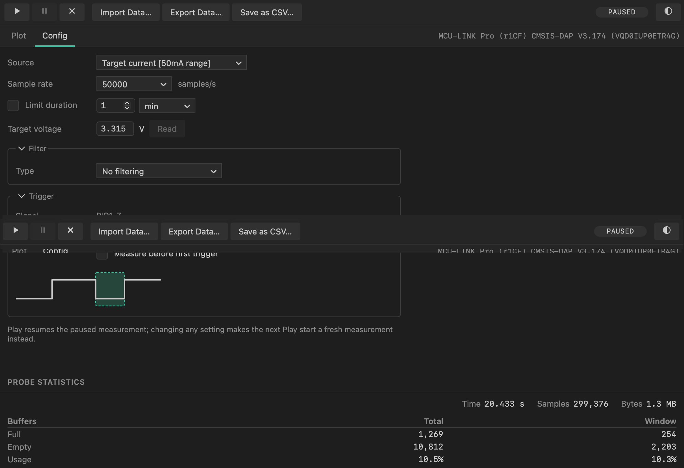
• Source: The quantity to measure. The list is populated from the capabilities that the connected probe advertises. For example, Target current [50 mA range], Target voltage, Target power, Debug interface VRef, or Analog input.

• Sample rate: Number of samples per second (10 kHz – 100 kHz).

• Limit duration: When checked, the measurement stops automatically after the specified time (hours, minutes, or seconds). When unchecked, it runs until you press Pause.

• Target voltage: The voltage used to derive power and energy for a current measurement. Type a value in volts, or press Read to sample the target-voltage source once and fill it in automatically.

• Filter: An optional noise filter applied to the samples, Moving Average, Arithmetic Mean, First-Order Low-Pass, or Kalman, with its relevant parameter. Select No filtering to disable. The filter can also be changed while imported data is displayed, letting you re-apply different filters to the same recording. Re-applying a filter re-processes every recorded sample. Therefore, on a long capture (an hour at 50 kHz is roughly 180 million samples) it takes about a minute. The progress is shown under the toolbar.

• Trigger: Optionally, gate the measurement on a probe input signal.

  • Signal: The probe GPIO monitored for triggering (for example PIO1_7), shown when the probe advertises a trigger input.

  • Mode: No trigger (measure continuously), Level High / Level Low (measure while the signal is high/low), or Pulse High / Pulse Low (each pulse toggles measurement on/off).

  • Measure before first trigger: Whether the measurement is active before the first trigger edge/pulse arrives.

Statistics

The lower part of the Config tab shows live transport statistics for the session:

• Time: Stream time elapsed on the probe.

• Bytes: Amount of data transferred from the probe.

• Samples: Number of samples collected.

• Buffers: Full/Empty read counts and their Usage ratio, reported both as a running Total and over a recent Window. A low usage ratio indicates that the host is comfortably keeping up with the probe’s data rate.

Plot tab

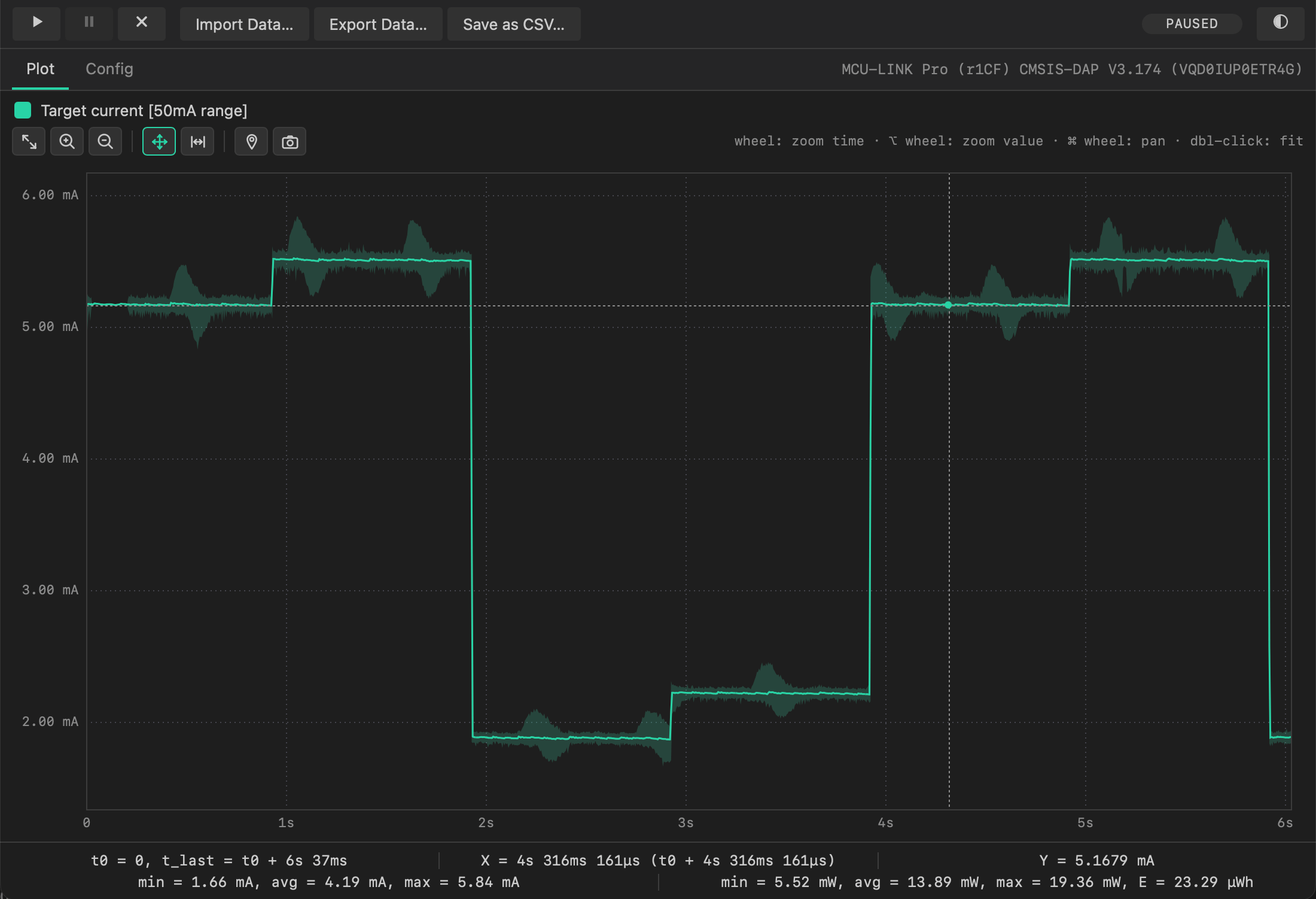
The Plot tab visualizes the measured quantity over time. During a capture, the plot updates live and auto-scales to follow the incoming data. When paused, the plot can be interacted with to explore captured data.

Plot area

The vertical axis shows the measured quantity in physical units and the horizontal axis shows time. A light-dotted grid snaps to round values to aid reading. The level of detail adapts to the zoom level:

• When zoomed out, each pixel column summarizes many samples: a lighter band shows the min–max range (the signal’s variation) and a bolder line/marker shows the average.

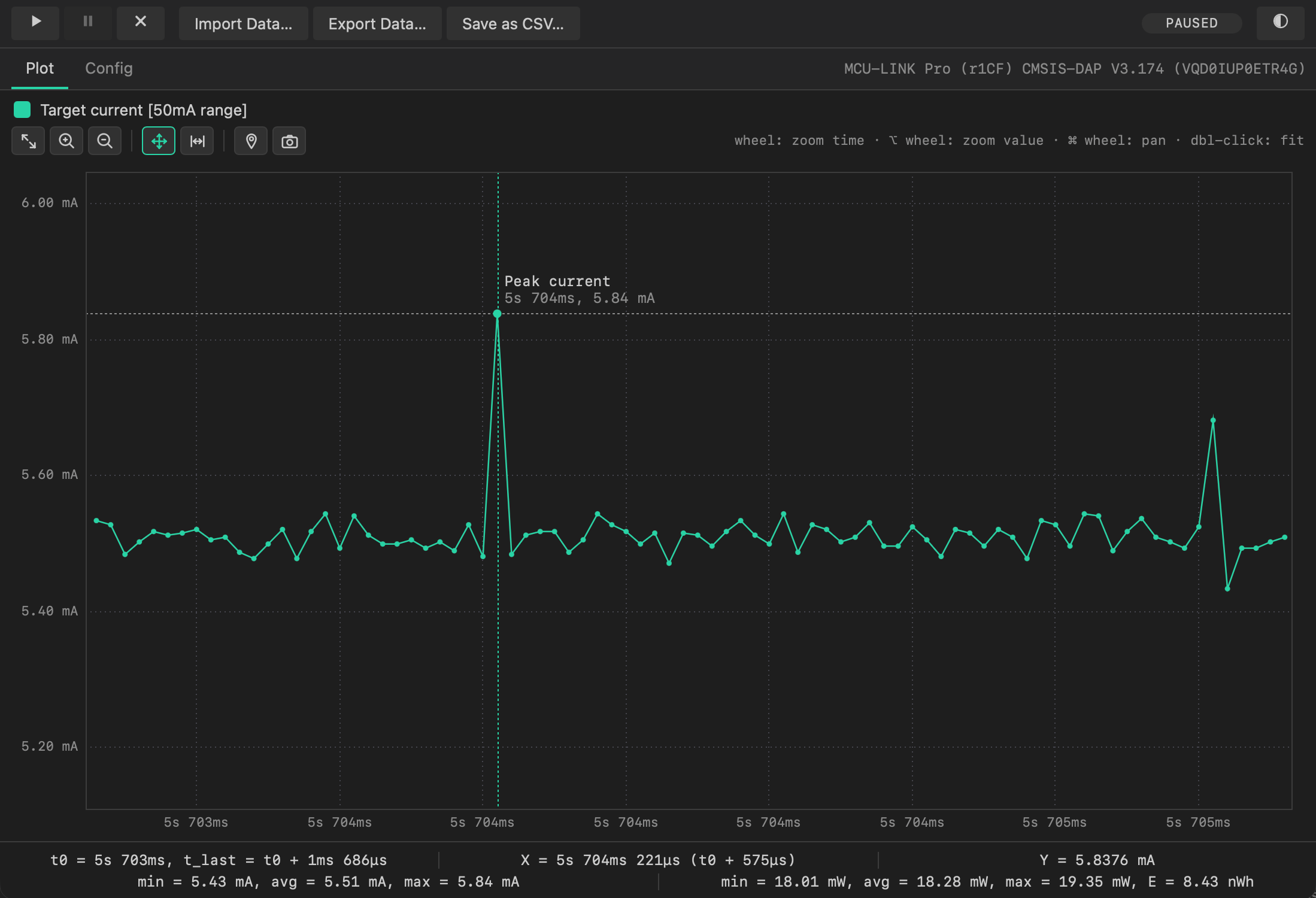
• When zoomed in far enough that individual samples are distinguishable, samples are drawn as points connected by lines.

Legend

A colored swatch and label above the plot identify the measured source (for example Target current [50 mA range]).

Status area

Two lines beneath the plot summarize the data:

• Top line: The plotted time range, the hovered X/Y value (shown while the pointer is over the plot), and while a range is selected the measured time span Measured Δt.

• Bottom line: The min/avg/max of the measured quantity and, when a target voltage is available, the corresponding power figures and the total energy (E).

The status figures reflect the data currently plotted, or the selected range when a selection is active.

Plot tools

After a capture is paused, the tool row above the plot becomes active:

• Autoscale: Fit all captured data into view (or double-click the plot).

• Zoom in/Zoom out: Zoom the time axis. The mouse wheel zooms as well.

• Pan: Drag to move the view. Space bar selects Pan mode.

• Measure/select: Drag to select a time range for analysis (see below).

• Annotate: Click a point to attach a note; click an existing marker to remove it.

• Save PNG: Save the current plot as a PNG image.

Mouse-wheel shortcuts (the modifier keys differ per OS: Alt/⌥ and Ctrl/⌘):

• Wheel up/down: Zoom the time axis in/out.

• Alt (⌥ on macOS) + wheel: Zoom the value axis.

• Ctrl (⌘ on macOS) + wheel: Pan the time axis.

• Double-click: Fit all data.

• Space bar: Switch to Pan mode.

Measuring a time range

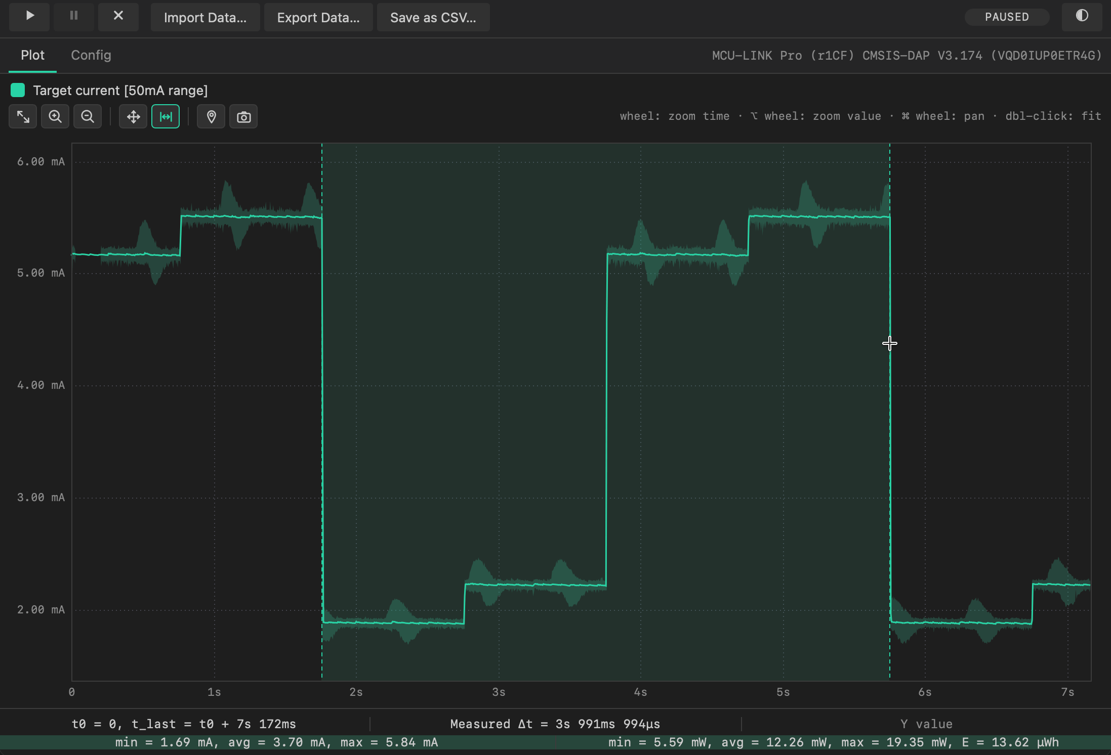
To mark a time range, select the Measure / select tool (or hold Shift) and drag across the plot. The selected span is highlighted, and the top status line displays Measured Δt, while the bottom status line updates. As a result, the min/avg/max, power, and energy figures apply only to the selected range. The highlighted background indicates that these values apply exclusively to the selected interval.

Exporting and importing data

Captured data can be saved for further analysis:

• Export Data… writes an Energy Measurement .zip archive containing the raw binary samples and a configuration descriptor. The same archive is produced by the report subcommand’s --output-bin option.

• Import Data… opens a previously exported archive and plots its data.

• Save as CSV… writes the scaled values in a human-readable format as CSV.

The binary Energy Measurement .zip format is fully compatible with the Import/Export data functionality in MCUXpresso IDE’s Energy Measurement view.

Offline mode (no probe)

All three subcommands can work on a previously captured archive without a probe connected, so a measurement can be analyzed anywhere — on a CI host, on a colleague’s machine, or long after the board was disconnected.

The capture settings are baked into the recording, so the source, sample rate, duration, trigger and target voltage cannot be changed offline. The noise filter is the exception: it is re-applied to the recorded samples, which makes it possible to compare filters on the same data.

Offline reporting (report --offline ARCHIVE)

./LinkServer measure report --offline session.zip replays a saved archive and prints the same report produced during a live capture:

Reporting Target current [50 mA range] (@ 50000 samples/s) for 3.465s.
Target current [50 mA range] duration: 3.465 s (173228 samples)
  min = 1.86 mA,  avg = 4.05 mA,  max = 5.84 mA
  min = 6.16 mW,  avg = 13.37 mW,  max = 19.28 mW  (3.30 V)
  E = 12.88 µWh

-i, --report-interval, --no-summary, -f, --filter, --output-csv, and --output-bin behave the same as they do for a live capture, allowing a recording to be re-reported, re-filtered, and re-exported:

./LinkServer measure report --offline session.zip --filter maf:16 --output-bin filtered.zip --output-csv filtered.csv

The archive and the CSV written above both contain the filtered samples, matching the report. Capture options that the recording already fixes (--source, --rate, --time, --voltage, --trigger, --trigger-initial, --probe) are ignored, with a warning naming them. Ctrl-C aborts the replay; no report is printed and no file is written.

Offline graphical interface (gui --offline / server --offline)

The gui and server subcommands accept --offline, which starts the interface without connecting to a probe. Live capture is disabled and the configuration form is replaced by a prompt. The only available action is Import Data…, therefore, you can open and analyze an Energy Measurement archive captured earlier or on another machine. All post-capture analysis (zoom, pan, measure, annotate, export) works as usual on the imported data.

./LinkServer measure gui --offline

--offline optionally takes the path to an Energy Measurement .zip archive, which is then loaded automatically when the interface opens; no need to browse for it with Import Data… afterward.

./LinkServer measure gui --offline capture.zip

In the standalone window, Import Data… opens a native file dialog. In server mode, the browser asks for the path to an archive on the server host. Similarly, Export Data… and Save as CSV… ask for a destination paths on the server host, with the path pre-filled with the directory from which the server was started.

Data files and disk usage

Energy Measurement stores captured samples in a compact and efficient Energy Measurement binary ($EMF) format. Raw ADC values interleaved with hierarchical min/avg/max summaries so the viewer can render any zoom level quickly. Export Data… and report --output-bin packages this binary together with a small configInfo.csv descriptor into a single .zip archive:

EnergyMeasurement_YYYYMMDDhhmm.zip
├── rawData.bin      # the $EMF sample stream
└── configInfo.csv   # probe, source, unit scaling and target voltage

CSV export (Save as CSV… / report --output-csv) instead writes scaled values as text: a timestamp_us column (integer microseconds relative to the first sample) and the measured value, plus a power_W column for a current source when a target voltage is available.

Disk usage

The binary format uses a fixed ~5.6 bytes per sample. Therefore, the on-disk size depends only on the sample rate and the capture duration — roughly 20 MB per hour for every 1 kHz of sample rate:

Sample rate	Approx. disk use per hour
10 kHz	~0.2 GB
25 kHz	~0.5 GB
50 kHz (default)	~1.0 GB
62.5 kHz	~1.25 GB
100 kHz	~2.0 GB

• In the graphical modes, every capture continuously streams to a temporary working file (at the rate above) so it can be explored and exported later. This space is reclaimed when you press Clear or close the interface. In report mode, sample data is written to disk only when --output-bin or --output-csv is given. The capture is recorded once into a temporary working file of the size above. The archive and/or the CSV are produced from it, and is removed when the command finishes.

• The exported .zip is compressed, so the saved archive is smaller than the working file (how much depends on how compressible the signal is).

• A CSV export is uncompressed text and is several times larger than the binary, typically requiring 3 GB to 6 GB per hour at 50 kHz, depending on the values.

Running out of disk space

The graphical interface (gui / server) watches free space and shows a banner across the top — red for a failure, amber for a warning:

• If free space is already below about 200 MB, a new capture does not start (the Play button is disabled) until space is freed.

• If space runs low while capturing, the capture is automatically paused so the data collected so far is preserved — free up space, then press Play to resume. This is the amber case: nothing is lost.

• If the drive fills completely mid-capture, the capture stops; free up space, then Export or Clear the data.

• Before an export or import begins, the required space is estimated. If insufficient space is available, the operation is refused up-front and reports both the required and available space. If a write operation still runs out of space, the incomplete file is automatically deleted to reclaim the occupied storage.

Dismiss a banner with the ✕ at its right; it also clears by itself when the next operation starts.

In report mode, there is no automatic pausing. If the drive fills while writing an archive or CSV, the capture ends with a measurement failed error. Make sure that the target volume has room for the expected size (see the table above) before starting a long capture.

Color theme

The graphical interface supports dark and light themes.

In gui mode, a theme-toggle button at the right end of the toolbar switches between them on the fly. The chosen theme is remembered and restored the next time the GUI is started.

The initial theme can also be set from the command line with --theme dark|light:

• In gui mode, --theme picks the starting theme. When it is omitted, the last theme used — set with the toggle button or a previous --theme — is restored, falling back to dark the first time.

• In server mode, --theme forces a theme for all connecting clients; when it is omitted, each client follows its own preference. The toggle button is not shown in this mode.

Examples

• Open the standalone GUI, pre-selecting the current source and a 3.3 V rail for power/energy:
  ./LinkServer measure gui --source current --voltage 3.3

• Same, using the top-level alias:
  ./LinkServer gui measure --source current --voltage 3.3

• Serve the interface to a browser in light theme:
  ./LinkServer measure server --source current --theme light

• Open the GUI to analyze a previously captured archive (use Import Data… once the window opens):
  ./LinkServer measure gui

• Open the GUI without a probe for inspecting an archive (offline mode):
  ./LinkServer measure gui --offline

• Open the GUI offline and load an archive automatically:
  ./LinkServer measure gui --offline capture.zip

Use ./LinkServer help measure for more information and options.